
In 1838 Friedrich Bessel announced the first reliable measurement of stellar parallax for 61 Cygni, proving that star distances could be measured rather than guessed.
Measuring distance matters for many reasons: spacecraft navigation, rendezvous planning, mapping our Galaxy, and testing cosmological models. Distances in astronomy span more than a dozen orders of magnitude, from laser-ranging a lander a few meters away to measuring objects billions of light-years distant. For a concrete anchor, 1 AU = 149,597,870.7 km.
Astronomers and engineers use a toolbox of roughly ten distinct, reliable methods to measure distances in space — from centimeter-scale laser ranging to billion-light-year cosmological probes — and each method fits a particular distance scale and application. Below I organize those techniques by practical scale and approach: geometric/direct ranging, astrometry, standard candles and empirical relations, and cosmological probes.
The overview that follows highlights the principles, typical precisions, and historical or modern examples (Apollo, DSN, Hipparcos, Gaia, HST, Cassini, GW170817) so you can see which method suits a given problem.
Geometric & Direct Ranging Methods
This category measures distance by timing electromagnetic signals or using direct geometry. It’s most accurate inside the solar system and to nearby spacecraft — from meters out to tens of astronomical units — and gives absolute, model-independent distances that mission planners rely on.
Typical precision ranges from centimeter-level (Earth–Moon) up to meters or kilometers for deep-space targets, depending on technique and geometry. Agencies such as NASA and ESA operate the instruments that make these measurements: ground radar, the Deep Space Network (DSN), and laser arrays at observatories.
These methods underpin spacecraft navigation, refine planetary ephemerides, and provide calibration anchors for other rungs of the distance ladder.
1. Radar and Laser Ranging
Radar or laser ranging sends short pulses toward a target and times the return; distance is c × time/2, where c = 299,792.458 km/s. That simple geometry gives an absolute range if you can detect the echo.
Radar observations of Venus in the 1960s dramatically improved the Astronomical Unit estimate and helped fix planetary orbits. Modern radar and laser systems can determine planetary distances to meter-level precision for nearby targets under good conditions.
Practical uses include improving planetary ephemerides, calibrating the AU, and supporting mission design to Mars and other targets; JPL and other centers routinely combine these ranges with optical astrometry and spacecraft tracking data.
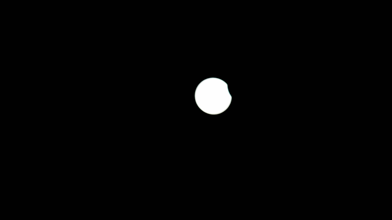
2. Lunar Laser Ranging and Planetary Transponders
Lunar laser ranging fires short laser pulses at retroreflectors left on the Moon (Apollo 11 placed the first in 1969) and times the return. Because the reflector returns a clean signal, current measurements reach roughly 1–2 cm accuracy in the Earth–Moon distance.
Those precise ranges test gravity (equivalence principle, inverse-square law), track tidal acceleration, and improve the Moon’s ephemeris — all useful for future landings and navigation. For interplanetary missions, active transponders on landers and orbiters allow two-way ranging with similar operational benefits.
Range data to Mars landers and orbiters, for example, feed into gravity models and navigation solutions used by mission teams at NASA/JPL and ESA when planning maneuvers and descents.
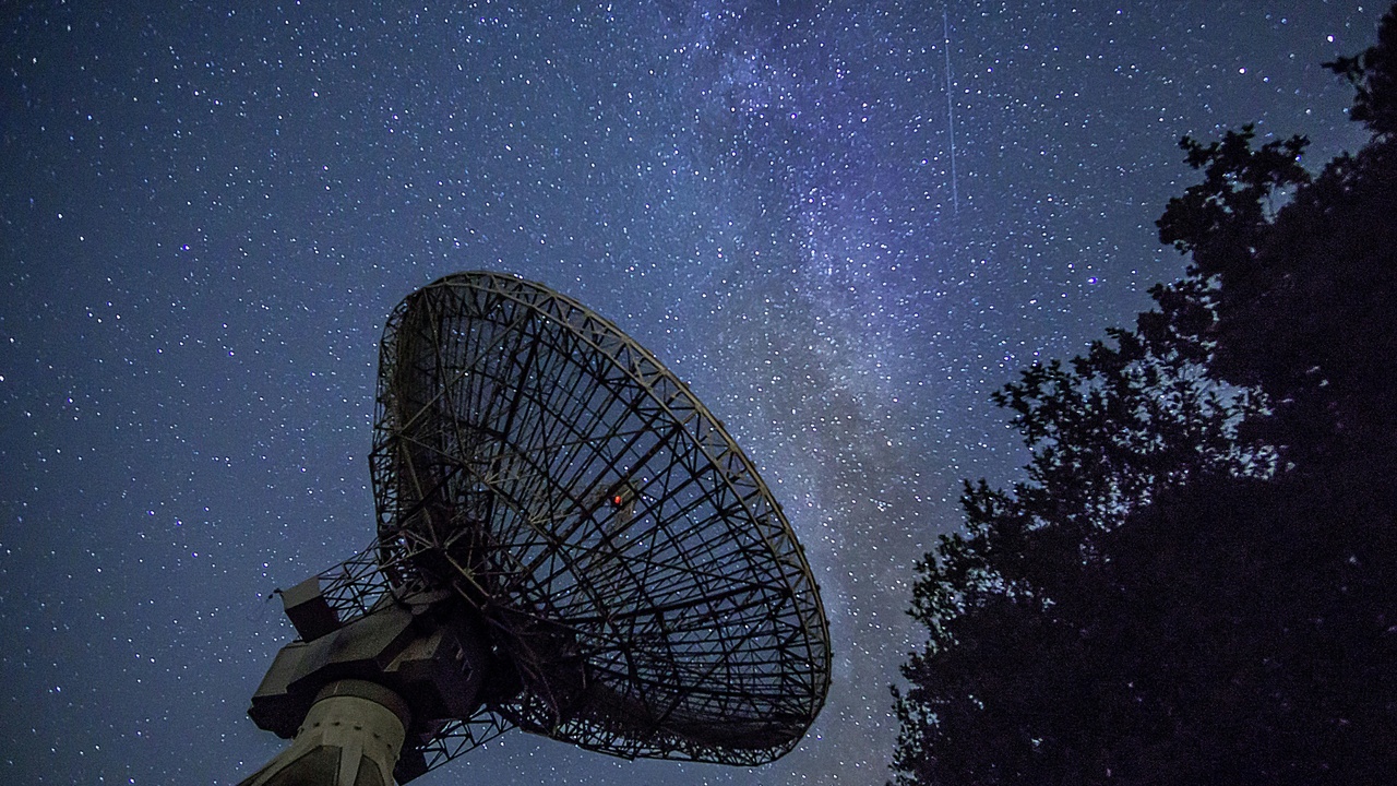
3. Spacecraft Two-way Ranging and Radio Tracking
The Deep Space Network performs two-way ranging and Doppler tracking to measure spacecraft range and radial velocity. Combining range with Doppler and multi-station angle measurements yields precise spacecraft state vectors.
DSN geometry and signal quality determine localization; for many missions the network can localize spacecraft to sub-kilometer precision at interplanetary distances. Teams used this for Cassini navigation at Saturn and for trajectory corrections on New Horizons before the Pluto flyby.
Those radio-tracking products are essential for safe navigation, targeting scientific observations, and refining gravity fields of planets and moons.
Astrometry and Geometric Parallax
Astrometry measures positions and apparent motions of stars against distant background sources. Parallax — the annual shift caused by Earth’s orbit — gives a direct geometric distance without astrophysical assumptions, making astrometry the foundation of the cosmic distance ladder.
Historically Bessel’s 1838 parallax proved stars are distant. Advances like Hipparcos (catalog published 1997) and ESA’s Gaia (science operations from 2016 onward) pushed precision from tens of milliarcseconds (mas) down to milliarcseconds and microarcseconds (μas), extending parallax reach from a few parsecs to many thousands.
Typical precision today ranges from mas for faint stars to tens of μas for bright sources, which lets us map the Milky Way, calibrate standard candles, and anchor extragalactic distances.
4. Classical Stellar Parallax
Stellar parallax is the apparent angular shift of a nearby star caused by Earth’s motion around the Sun. The relation is simple: distance in parsecs equals 1 divided by the parallax angle in arcseconds (d = 1/p).
Bessel’s 1838 measurement of 61 Cygni started the field; by definition 1 parsec is the distance that gives a parallax of 1 arcsecond, about 3.26 light-years. Historically, ground-based parallax work was limited to tens of milliarcseconds, so it covered only nearby stars.
Because parallax is geometric and model-independent, it provides the first rung that calibrates Cepheids and other standard candles used for greater distances.
5. High-Precision Astrometry (VLBI, Gaia)
Very Long Baseline Interferometry (VLBI) and space missions like Gaia push parallax precision into the microarcsecond regime for selected targets. VLBI gives μas-level positions for radio sources and masers, while Gaia DR2/EDR3 measured over a billion stars with precisions down to roughly 20–30 μas for bright stars.
That leap in precision extends reliable geometric distances to star-forming regions across much of the Galaxy and tightens calibrations for Cepheids and RR Lyrae. The result: fewer systematic errors when those calibrated candles are used to measure extragalactic scales.
VLBI maser parallaxes have mapped spiral-arm structure directly, and Gaia’s catalogs are publicly accessible for researchers and amateur sleuths alike.
Standard Candles and Empirical Relations
When parallax can’t reach, astronomers infer distance by comparing an object’s observed brightness to its intrinsic brightness or another measurable property. These standard candles and empirical relations bridge kiloparsecs to hundreds of megaparsecs, but they require good calibration—often from parallax or other geometric anchors.
Henrietta Leavitt’s discovery of the Cepheid period–luminosity relation in 1912 provided the first reliable extragalactic ruler. Modern methods typically yield per-object uncertainties around 5–15% after calibration, depending on the indicator and data quality.
Used together, these relations build large distance catalogs that let us measure galaxy environments, Hubble’s constant, and the expansion history of the Universe.
6. Cepheid Variables and the Period–Luminosity Law
Cepheid variables are pulsating stars whose pulsation period tightly correlates with intrinsic luminosity—a relation discovered by Leavitt in 1912. Measure the period, infer the absolute magnitude, compare to observed magnitude, and you get distance.
Well-calibrated Cepheids (using HST and Gaia parallaxes) can reach tens of millions of light-years with uncertainties around 5–10% per object. Edwin Hubble used Cepheids in the 1920s to show Andromeda lies far outside the Milky Way.
Modern infrared observations reduce dust effects and improve the period–luminosity zero point, making Cepheids a reliable rung for measuring the local expansion rate.
7. Type Ia Supernovae (Standardizable Candles)
Type Ia supernovae arise from thermonuclear explosions that reach a consistent peak luminosity. Empirical light-curve corrections standardize them so a single event can give a luminosity distance with roughly 7–10% precision after calibration.
Because they’re bright, Type Ia supernovae can be seen to redshifts z ≈ 1–2. The 1998 discovery—by teams led by Perlmutter, Riess, and Schmidt—that distant Type Ia appeared dimmer than expected revealed the accelerating expansion of the Universe and brought dark energy into focus.
Surveys that find and follow many SNe Ia remain central to measuring H0 and constraining cosmological parameters when combined with calibration from Cepheids and geometric anchors.
8. Tully–Fisher, Surface Brightness Fluctuations and Other Empirical Relations
Empirical scaling relations fill gaps where standard candles aren’t available. The Tully–Fisher relation ties a spiral galaxy’s rotation speed (measured from HI 21-cm line widths) to its luminosity, letting you infer distance for tens to hundreds of Mpc.
Surface brightness fluctuations (SBF) measure pixel-to-pixel brightness variance in elliptical galaxies to infer distance at intermediate ranges (~10–100 Mpc). Both methods need careful corrections for inclination, population differences, and extinction.
Using near-infrared photometry and high-quality rotation curves reduces scatter, so these relations are useful for building large, homogeneous catalogs of galaxy distances for environmental studies and H0 work.
Redshift, Lensing, and Gravitational-Wave Probes
These methods are designed for extragalactic and cosmological scales — from tens of megaparsecs to the observable horizon. They often depend on a cosmological model to translate observables into distances, but they reach much farther than any geometric method alone.
Modern cosmology combines redshift surveys, Type Ia supernovae, lensing time delays, and gravitational-wave events to cross-check systematics and measure parameters like H0 (currently reported in the range ≈ 67–74 km/s/Mpc, a notable tension).
Two emerging, independent probes — strong-lens time delays and gravitational-wave “standard sirens” — provide model-independent distance information in select cases, helping to break degeneracies in cosmological analyses.
9. Redshift and Hubble’s Law (Cosmological Distances)
At low redshift, a galaxy’s recessional velocity is approximately v = H0 × d, so measuring redshift gives a distance estimate via Hubble’s Law. Edwin Hubble first established this relation in 1929, and refinements since then have tightened the constants and methods.
At higher redshift you must use a full cosmological model (ΛCDM or alternatives) to convert redshift into comoving, angular-diameter, or luminosity distance; that conversion depends on H0, the matter density, dark energy properties, and curvature.
Redshift-based distances power large surveys (SDSS, DESI) that map large-scale structure and measure lookback time; but remember that a systematic shift in H0 shifts all derived distances, so independent anchors remain crucial.
10. Gravitational Lensing Time Delays and Gravitational-Wave ‘Standard Sirens’
Strong gravitational lenses produce multiple images of a background source with different light-travel times. Measuring those time delays and modeling the mass distribution yields distances and an H0 measurement; projects like H0LiCOW have achieved ~3–7% precision on H0 from selected systems.
Gravitational-wave events act as “standard sirens”: the waveform encodes the absolute luminosity distance without relying on astrophysical distance ladders. The binary neutron-star merger GW170817 (August 2017) gave a distance of roughly 40 Mpc and an independent H0 estimate when its electromagnetic counterpart provided the redshift.
Both lensing and GW methods are powerful cross-checks because they don’t share the same systematics as Cepheids or supernovae, though they require high-quality data (time-delay monitoring, lens models, or EM counterparts) to reach competitive precision.
Summary
- Different techniques cover different scales, from centimeter-level lunar laser ranging to billion-light-year cosmological probes; each method fits a particular practical need.
- Direct geometric methods — radar/laser ranging and parallax (Gaia, VLBI) — provide absolute anchors that calibrate empirical tools like Cepheids, Type Ia supernovae, Tully–Fisher, and SBF.
- Emerging independent probes such as lensing time delays and gravitational-wave standard sirens (GW170817 ≈ 40 Mpc) offer powerful checks on the distance scale and the H0 tension.
- Surprising contrasts: lunar laser ranging measures the Earth–Moon distance to centimeter precision, while Type Ia supernovae and redshift allow us to measure cosmic expansion across billions of light-years.
- If you want to explore further, check the Gaia catalogs for parallaxes or NASA/ESA mission pages for DSN, Apollo, and GW follow-up data — or try a simple parallax calculation using d = 1/p (pc) with a nearby star.
Enjoyed this article?
Get daily 10-minute PDFs about astronomy to read before bed!
Sign up for our upcoming micro-learning service where you will learn something new about space and beyond every day while winding down.


